1 Abstract
This report presents an analysis of fluorescence excitation-emission matrix (EEM) spectroscopy data from natural water and wastewater samples. The work began as an exploratory study of the data, with a focus on understanding its basic structure and variation. The primary research question investigated is whether EEM spectroscopy can be used to infer organic micropollutant (OMP) spiking metadata and sample origin. A preprocessing and dimensionality reduction pipeline was developed, group structure was analyzed using permutation testing, and predictive models were used for concentration regression and source classification. The report also includes a conditional generative model that attempts to reconstruct plausible EEM surfaces from metadata. Results indicate that the reduced features preserve meaningful structure, that source groups are significantly separated, and that the predictive models perform well with complementary strengths.
2 Introduction
The dataset contains fluorescence EEM measurements for organic micropollutants in natural water and wastewater. An excitation-emission matrix is a grid of fluorescence intensity values measured across excitation and emission wavelengths. Organic micropollutants are trace chemical contaminants, such as pharmaceuticals, that can appear in aquatic environments.
The target micropollutants are ciprofloxacin (cip), naproxen (nap), and zolpidem (zol). The modeling goals are threefold: regression to predict cip, nap, and zol concentrations; multiclass classification to identify the source group of a sample; and binary classification to determine whether a sample is spiked at all. Dissolved organic matter (DOM) also causes fluorescence that overlaps with the micropollutants in the EEM data, which makes detecting the micropollutants more difficult.
A shared preprocessing and dimensionality reduction pipeline was used to convert raw EEM grids into compact principal component features, then evaluate two predictive model families. The first is a multitask multilayer perceptron (MLP), which is a neural network composed of stacked layers of weighted sums and nonlinear activations. The second is a random forest, which combines many decision trees and averages their outputs for stable prediction. We also implement a conditional generative model that synthesizes EEM grids from metadata and source category, providing a complementary, model-based view of the learned fluorescence patterns.
The work is grounded in the source study[1] that introduced the dataset and demonstrated fluorescence-based measurement and analysis of the water samples using PARAFAC modelling.
3 Methods and Models
This section describes the data processing steps, the statistical testing framework, and the predictive model families evaluated in the project. The aim is to explain what was done, why it was done and how each step connects to the next.
Preprocessing of EEM Data
The dataset contains EEM measurements for OMP standards, natural waters, and wastewater samples collected in June and November. Each EEM is stored as a comma separated values (CSV) file with emission wavelengths as rows and excitation wavelengths as columns. Metadata files list sample identifiers, concentrations (conc_cip, conc_nap, conc_zol, in g/L), and descriptive labels such as natural water or wastewater influent and effluent. These metadata provide the supervised targets used in regression and classification.
The raw EEMs provided in the dataset were already corrected using standard fluorometric procedures from the source study, including instrument excitation and emission corrections, blank subtraction, and inner filter effect correction. Signals were normalized to the Raman peak area of ultrapure water, and scatter bands were removed and replaced with missing values.
Raw EEMs contain missing values around scatter bands and vary slightly in wavelength grids. All EEMs were standardized to a common grid by taking the intersection of wavelength axes across files. Missing values introduced by scatter removal showed up in the CSV files as NaN, which means “Not a Number”. These missing values were filled via smooth linear interpolation to provide a consistent feature layout for subsequent dimensionality reduction and model training.
Core preprocessing was performed using Pandas[2], a tabular data library, with functions such as pandas.read_csv(), and NumPy[3], a numerical computing library, with SciPy[4] interpolation via scipy.interpolate.griddata().
Visualization of EEM Data
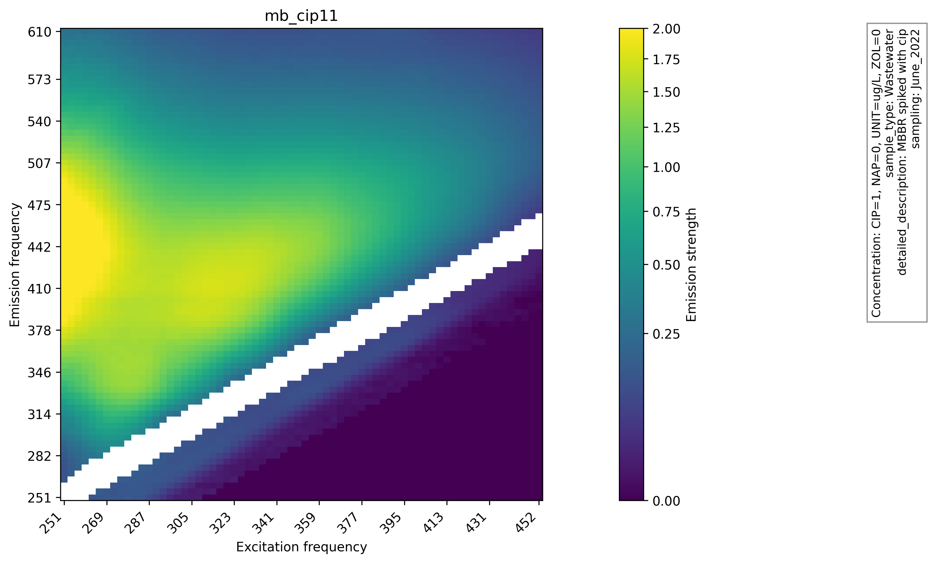
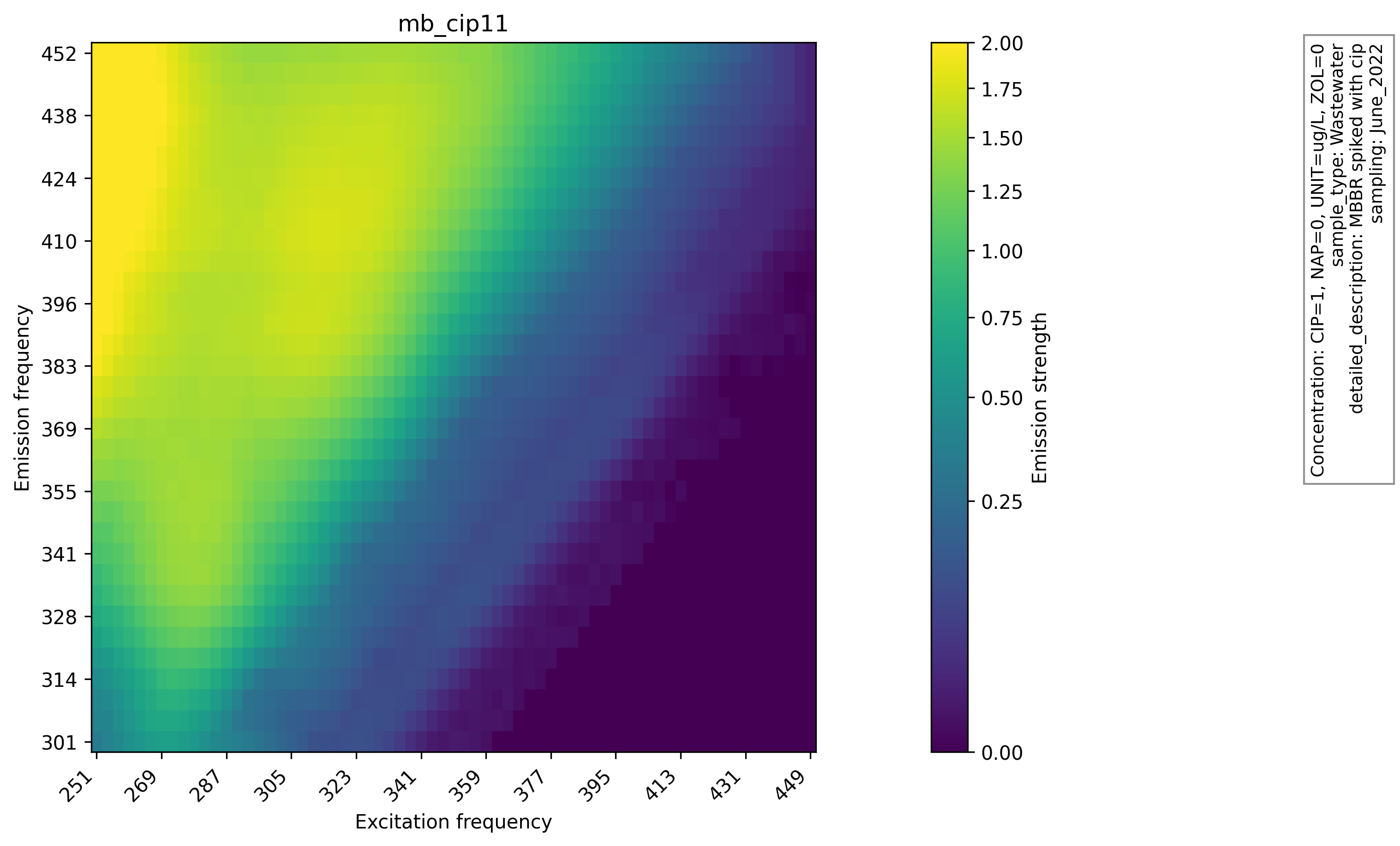
Heatmaps of raw and preprocessed EEMs were generated to visually inspect the effect of interpolation and scatter handling. The heatmaps of raw EEMs show scatter gaps and uneven intensity near the diagonal. After preprocessing, the filled regions are smooth and the overall fluorescence patterns remain intact. This comparison supports the choice of interpolation and indicates that the preprocessing step preserves the global structure required for downstream analysis, and the raw EEM heatmap with scatter gaps and the same sample after preprocessing are shown below. Plots are produced with Matplotlib[5] using functions like matplotlib.pyplot.imshow().
Principal Component Analysis (PCA)
Each preprocessed EEM is flattened into a feature vector and subjected to PCA. Principal component analysis is a linear technique that projects data into orthogonal (perpendicular) directions that capture the largest variance.
10 principal components were retained, which capture 99.93% of the total variance. This compresses each EEM into a small, stable feature set while preserving the dominant structure needed for prediction and visualization.
The PCA computation uses NumPy linear algebra with numpy.linalg.svd(). Here SVD stands for “Singular Value Decomposition” and this function is used because PCA is calculated as the SVD of the data matrix.
Visualization and Interpretation of PCA Results
Two dimensional and three dimensional PCA plots were created, as well as an interactive plot with metadata on hover, and a three-dimensional PCA visualization of the sample groups is shown below. These visualizations verify that structure in the raw data is preserved after preprocessing and PCA. Interactive plots are produced with Plotly[6] using plotly.graph_objects.Scatter3d().
PCA plots reveal distinct clusters and curved trajectories. In the interactive plot, points along these trajectories can be seen to correspond to systematic changes in cip, nap, and zol concentrations, suggesting that the principal components preserve chemical variation rather than only noise.
These patterns are consistent with the idea that EEM fluorescence captures both source specific background signals and spiking related signals. The principal components appear to separate these effects, which makes them useful inputs for downstream models.
The exploratory phase was essential because it guided which modeling tasks were realistic. The clear structure in the reduced space suggested that both classification and regression would be feasible, which justified the later focus on predictive modeling.
Permutation Testing
A permutation test is a non-parametric statistical method for testing whether two groups are significantly different regarding a chosen statistic. The core idea is to compare the observed statistic to a large sample of alternate statistics obtained by repeatedly shuffling group labels. Because the labels are randomly reassigned, this sample represents the null hypothesis that group membership does not matter. This approach avoids assumptions about normality or equal variances, which can be hard to justify for fluorescence data.
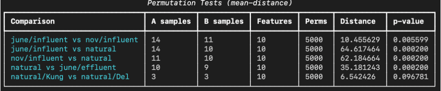
In this project, the statistic is the distance between the mean PCA vectors of the two groups. This statistic is simple and interpretable, and a large observed distance suggests that the groups occupy different regions of the reduced feature space, while a small distance suggests overlap. 5000 random relabelings were performed for each comparison and a p value was computed as the fraction of permuted distances greater than or equal to the observed distance. A small p value indicates that the observed separation is unlikely under random grouping. This test was applied to unspiked subsets of the data to isolate baseline source differences without spiking effects, which prevents concentration gradients from dominating the group comparison.
The test is implemented by concatenating samples from the two groups, shuffling the combined set, splitting it back into two groups of the original sizes, and recomputing the mean distance. This loop produces the null distribution of distances. The procedure is repeated for multiple group pairs, which enables the identification of which sources are clearly separated and which appear similar. A simple illustration of permutation testing is shown below.
Permutation testing is descriptive rather than predictive, and it complements the machine learning models. It provides a statistical check to confirm that the features contain real group differences before attempting to build models that exploit those differences to predict the metadata.
Because the test uses randomization, the p value can vary slightly between runs. A sufficiently large number of permutations was used to make this variability small relative to the effect sizes observed. The p values reported in the results section are therefore stable indicators of separation for the comparisons tested.
The permutation test also offers a way to interpret effect sizes. Larger observed mean distances indicate greater separation in the reduced space. When such distances coincide with small p values, the group differences are both statistically reliable and practically meaningful.
It is important to note that permutation testing does not explain why groups differ, only that they do. That is one reason to build predictive models, which help quantify how much information about spiking and source is contained in the EEM features.
A practical benefit of the permutation test is that it uses the same reduced features that feed the models. This means that the statistical test is directly tied to the features that the models rely on, so the two analyses reinforce each other rather than speaking about different spaces.
The permutation tests show that most source comparisons are significantly separated in PCA space, with the only non-significant comparison being between two natural water sources, likely due to similarity and small sample size. These results (shown below) support the interpretation that the reduced EEM features encode meaningful differences between sample origins.
Grid Search
The performance of multilayer perceptron and random forest models both depend on how certain parameters are chosen. These parameters that affect model performance, but must be determined before the model training process, are often called “hyperparameters” to distinguish them from any other parameters that are learned from data during training.
Grid search is a common way to find good hyperparameters. It works by evaluating a predefined set of parameter combinations and selects the best performing configuration according to a chosen metric. It provides a systematic way to explore tradeoffs such as model capacity, learning rate, or tree depth, and it makes the selection process transparent and repeatable. The alternative, manual tuning, is more subjective, less reproducible, and is likely to miss the best hyperparameter combinations.
Grid search has a computational cost because the number of combinations can grow quickly. To keep the search tractable, the focus was kept on ranges that are plausible given the dataset size and model complexity. For example, a moderate range of tree depths and hidden layer sizes were searched rather than extremely large values that would be unlikely to generalize.
5-Fold Cross Validation
An important consideration when training and evaluating models is which data the model should be trained on and which data it should be tested on. It is problematic to evaluate the performance of a model based on the data it has been trained on because models often memorize the training data and fail to generalize to new data. This is called “overfitting” and because of it, datasets are typically split into distinct training and testing sets where the model is only trained on the training set and tested on the testing set. This is also often extended with a “validation set” that is used as evaluation for iterative improvement of hyperparameters to preserve a testing set that has not been optimized for, even by hyperparameter selection. An alternative to this approach is to use 5-fold cross validation.
In 5-fold cross validation the dataset is split into five equal parts, called folds. The model is trained on four folds and tested on the remaining fold, and this is repeated so each fold serves as the test set once. Final performance is the average across the five test results. The concept of 5-fold cross validation is demonstrated in the video below.
This approach reduces dependence on any single train test split and provides a more reliable estimate of generalization performance. It is especially important when class sizes are imbalanced or when the dataset is modest in size, because a single split can overrepresent or underrepresent important groups.
We use stratified splitting when classification labels are involved so that each fold preserves the class distribution as much as possible. This keeps training and validation sets comparable and avoids misleading accuracy estimates. It also ensures that rare categories are present in both training and validation across folds. 5-fold cross validation is a balance between statistical reliability and computational cost. Using more folds would provide more training data in each split, but it would also increase computation time. For instance, for small datasets, sometimes “leave-one-out cross validation” is used where every datapoint is in its own fold. Five folds provides a stable estimate while keeping the workflow manageable.
Neural Network and Multilayer Perceptron Models
A neural network is a learnable function that changes its shape to fit a set of input and output data. It is built from layers of weighted sums followed by non-linear activation functions, and the concept is shown here:

A multilayer perceptron (shown below) is the simplest form of neural network in which layers are fully connected and information flows forward from input to output.

The MLP is appropriate for fluorescence-based prediction because it can represent smooth non-linear relationships between principal component features and targets. It also supports multitask learning, which means a single model can predict concentrations and classifications simultaneously. This shared representation can improve efficiency and capture relationships between tasks, such as how spiking levels relate to source category.
The MLP is trained by minimizing a combined loss that includes regression error (MSELoss()) for concentration outputs and classification error (CrossEntropyLoss()) for categorical outputs. The model uses PyTorch[7] components such as torch.nn.Linear() and torch.utils.data.DataLoader() to define layers and manage training batches.
The multitask setup requires balancing losses so that the regression and classification objectives both improve. The final architecture uses multiple hidden layers with non-linear activations to capture complex relationships while keeping the model small enough for the dataset size.
Grid search over the following MLP hyperparameters was performed: learning rate (2e-3, 1e-3, 7.5e-4, 5e-4, 1e-4), hidden layer sizes ("32,16", "64,32,16", "128,64,32", "256,128,64"), batch size (16, 32, 64), optimizer (stochastic gradient descent (SGD) or Adam), and whether or not we performed a log transformation of the concentration targets.
A log transform of concentration targets was considered to reduce the influence of large concentration values to help the model treat proportional errors more evenly across the concentration range and stabilize training when targets span orders of magnitude. While the best reported configuration did not rely on the log transform, the option remained useful for alternative settings. From an implementation perspective, the network uses small fully connected layers rather than convolutional layers because the input is already condensed into principal components (even if PCA had not been used, convolutional networks would not necessarily be suitable because the input EEM data is not translation invariant). This makes the model compact and efficient, which is important for repeated training during grid search and cross validation.
Conceptually, the MLP learns to reshape the input space so that patterns related to spiking and source become easier to separate. It does this by iteratively making small updates to its parameters in the direction that locally minimizes error on the training data. This process is called gradient descent, and when it is performed using only a subset of the training data for each update, it is called stochastic gradient descent. A visual illustration is shown below. This ability is central to why it outperforms the random forest on regression, where smooth relationships matter more (as seen in Section 4).

Random Forest Models
A random forest is an ensemble of decision trees that vote to make the final prediction for the random forest model. Each tree learns a set of simple “if-then” rules that partition the feature space, and the forest aggregates predictions across trees to reduce variance and improve generalization. For regression, the output is the average of tree predictions, and for classification, the output is the majority vote.
Decision Trees
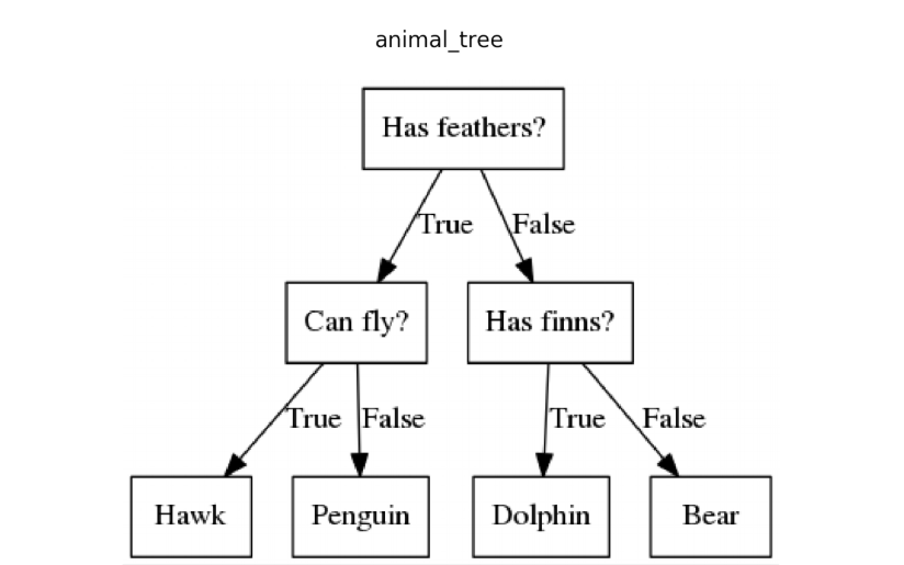
A decision tree is a hierarchical model that recursively splits the feature space using simple rules, such as thresholds on a single feature. Each split aims to reduce prediction error for regression or increase class purity for classification. The resulting model is interpretable because each path from root to leaf corresponds to a clear sequence of rules. Decision trees can overfit when allowed to grow deep, but they capture non-linear decision boundaries without requiring feature scaling. A simple visual example of a decision tree is shown below.
Random Forests as Ensembles of Decision Trees
Random forests are well suited to tabular data and perform reliably with moderate sample sizes. Because principal component features are already compact and informative, the random forest provides a strong baseline that is less sensitive to scaling or monotonic transformations. It is also easier to train and can be robust to noisy features.
Separate random forest models were used for regression and classification tasks. Grid search and 5-fold cross validation are used to select hyperparameters such as the number of trees (100, 200, 300, 400, 500) and maximum depth (None, 10, 20, 30, 40). The implementation of random forests uses scikit-learn[8] functions such as sklearn.ensemble.RandomForestRegressor() for the regression and sklearn.ensemble.RandomForestClassifier() for the classification.
Random forests can also provide feature importance measures, which are useful for understanding which principal components contribute most to the predictions. While interpretability was not the primary focus in this project, the availability of such diagnostics is a practical advantage of tree-based models and can guide future analysis.
Random forests can struggle with very smooth response surfaces because each tree produces piecewise constant predictions. This is one reason the random forest shows weaker regression performance compared to the MLP, even though its classification accuracy is strong.
In practice, the random forest tends to be more stable across different hyperparameters than the MLP. This makes it a useful benchmark model and a good option when the dataset is small or when robust classification is the main goal.
Another strength of the random forest is its resistance to overfitting when properly tuned. By averaging over many trees that each see slightly different data, the forest smooths out noise and focuses on the consistent patterns that appear across samples.
Model Selection
The MLP was used because fluorescence patterns and concentration effects are expected to vary smoothly and non-linearly in the reduced space. A single network predicts three concentrations, a categorical source label, and a spiked or not spiked flag. This joint setup encourages shared representations across tasks. The trade-off is sensitivity to preprocessing and hyperparameters, and the risk of overfitting on small datasets.
The random forest was used because it is robust on tabular features and performs well with limited sample sizes. It also provides a strong baseline for classification. The downside is that it does not model smooth gradients as directly as the MLP, and separate models are needed for regression and classification.
Both model families are implemented in Python. The MLP uses the PyTorch deep learning library with functions such as torch.nn.Linear() and torch.utils.data.DataLoader(). The random forest models use scikit-learn, a machine learning library for Python, with functions such as sklearn.ensemble.RandomForestRegressor(), sklearn.ensemble.RandomForestClassifier(), and sklearn.model_selection.GridSearchCV().
Model selection was driven by the data and the research goals. The MLP is preferred when the main objective is accurate concentration regression, while the random forest provides a robust option for classification and a useful comparison baseline.
Because the two model families capture different kinds of relationships, their combined results strengthen the overall conclusions. When both models agree on classification outcomes, confidence that the source signal is robust is gained. When they differ on regression outcomes, insight is gained into the importance of smooth non-linear modeling for concentration prediction.
The choice to include both models also fits the educational goal of comparing different modeling philosophies. The MLP represents a flexible, data driven approach, while the random forest represents a structured ensemble approach with more built-in interpretability.
4 Model Evaluation
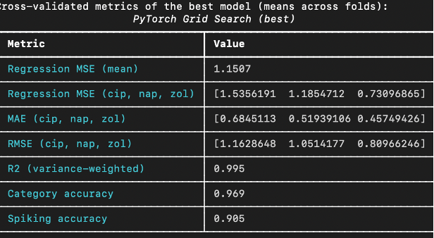
The best MLP from grid search achieves strong regression and classification results on cross validation. The values of the metrics are shown below.
In addition to evaluating the model based on its overall performance, it was also evaluated in a more interactive manner. After training the best 5-fold cross validation models, one of these models was interactively probed on its individual testing data samples. The excellent results of one such interactive prediction are shown below.
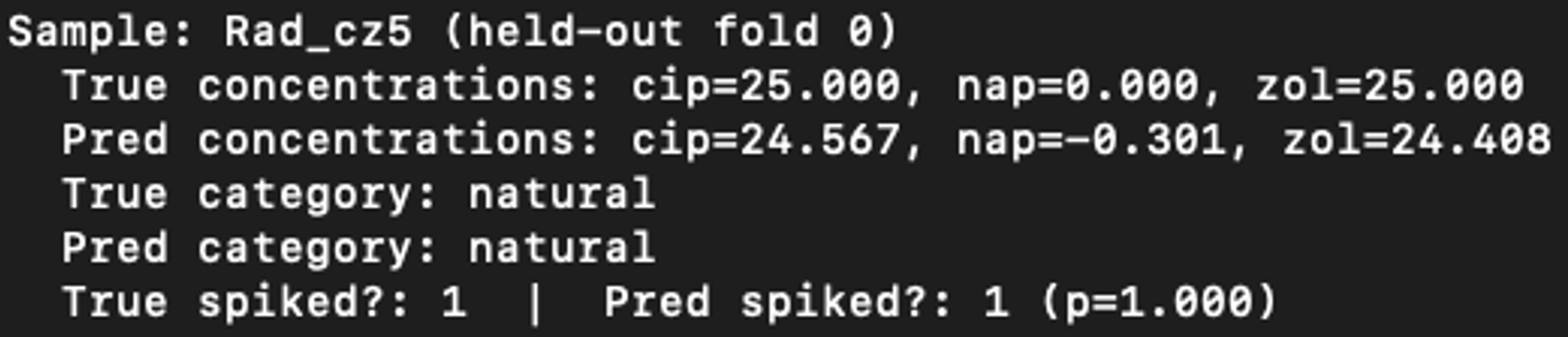
The mean absolute error (MAE) for cip, nap and zol concentrations are all around 0.5, which indicates that the MLP has at least learned to distinguish high levels of spiking from low levels. Another very important metric is the coefficient of determination (R2). The value of 0.995 means that only ½ of a percent of the variance of the spiking concentrations is not accounted for by the model’s regression output. Also note the 96.9% accuracy in sample source classification and the 90.5% binary spiking prediction accuracy. These values indicate excellent regression performance and strong classification accuracy.
The results from the best random forest model (shown below) demonstrated complementary strengths.
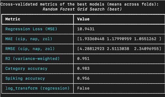
Compared to the MLP, the random forest is weaker for regression (slightly lower R2 of 0.951) but slightly stronger for classification tasks (category and spiking accuracy with 98.3% and 95.6%), which aligns with expectations for tree ensembles on tabular features.
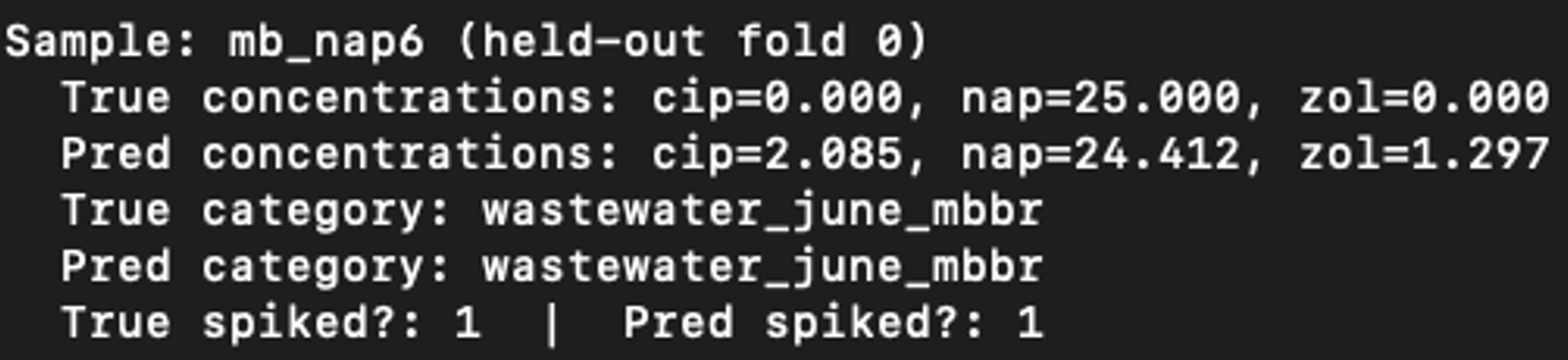
As was done for the MLP, an interactive prediction session was performed with the random forest model. An example is shown below. While this sample is not the same as the MLP example, the concentration predictions are less accurate for the random forest model.
The MLP is the better choice when concentration prediction is the priority, as evidenced by much lower MSE, MAE, RMSE and higher R2. The random forest excels on classification, likely due to its robustness to class boundaries in the reduced feature space. Across both models, zol appears easier to predict than cip, which suggests clearer fluorescence signatures for zol. Overall, both models show strong promise, with complementary strengths that could be leveraged depending on the application.
The classification metrics are high for both model families, which indicates that the source categories are well separated in the reduced feature space. The regression metrics show a larger gap between the MLP and random forest, suggesting that smooth non-linear modeling is more important for accurate concentration prediction.
When interpreting the regression metrics, it is important to remember that the units are g/L. Errors of 1-2 g/L can be meaningful in low concentration regimes, and therefore absolute errors should be interpreted alongside the underlying concentration ranges.
The evaluation results also reflect the challenges of multitask learning. The MLP must balance three regression outputs with two classification outputs. Achieving strong performance across all tasks suggests that the model is capturing shared structure rather than memorizing noise.
The evaluation also suggests that different metrics highlight different strengths. The random forest has excellent accuracy for classification tasks, which is valuable for source identification. The MLP has much lower regression error, which is essential for estimating concentrations.
5 Generative Modeling
After this project was presented, it was extended by training a conditional generator that maps metadata (cip, nap, zol concentrations) and source category to a reconstructed EEM grid. This model treats the EEM as the output and learns a direct mapping from metadata to fluorescence surfaces. Its role is complementary rather than competitive because it helps interpret how metadata might shape the full spectrum, which cannot be seen from reduced features alone.
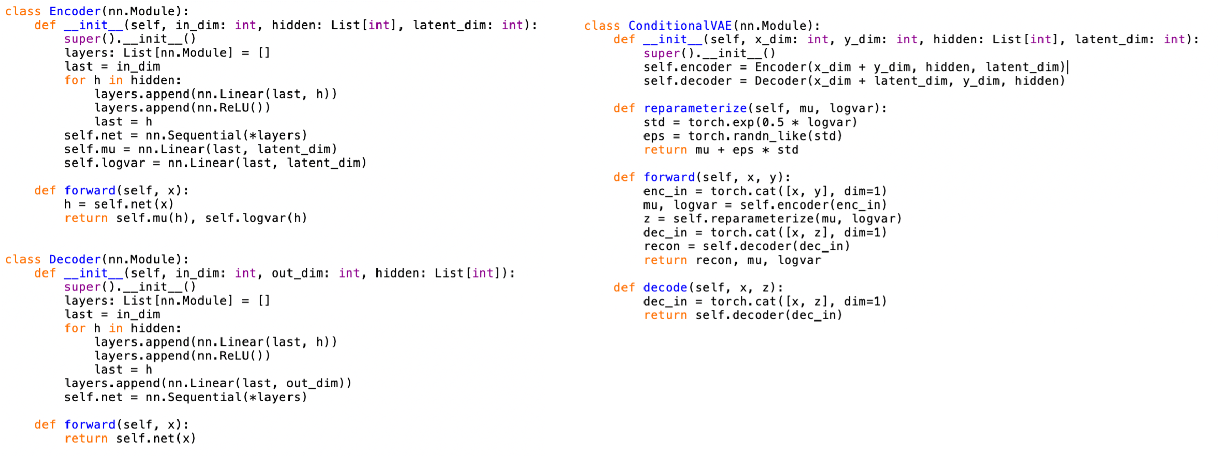
The generator is implemented as a conditional variational autoencoder in PyTorch in Python and uses the same preprocessed EEM grids as targets. Inputs include concentrations and a one hot encoding of sample source. The output is a reconstructed intensity grid that can be reshaped into an EEM. The model provides a qualitative check of whether metadata can reproduce observed fluorescence patterns and serves as a foundation for future, more rigorous generative evaluation. A screenshot of the most relevant PyTorch code is shown below.
Training a generator requires careful normalization because EEM intensities span a wide range. The same normalization and preprocessing conventions were used as for the predictive models to maintain consistency between inputs and targets. This allows direct visual comparison between generated and observed EEMs
An example of an excitation-emission matrix generated by this generator is shown below. This example was generated as wastewater from June in the influent with a cip spiking concentration of 50, and a nap concentration of 20.
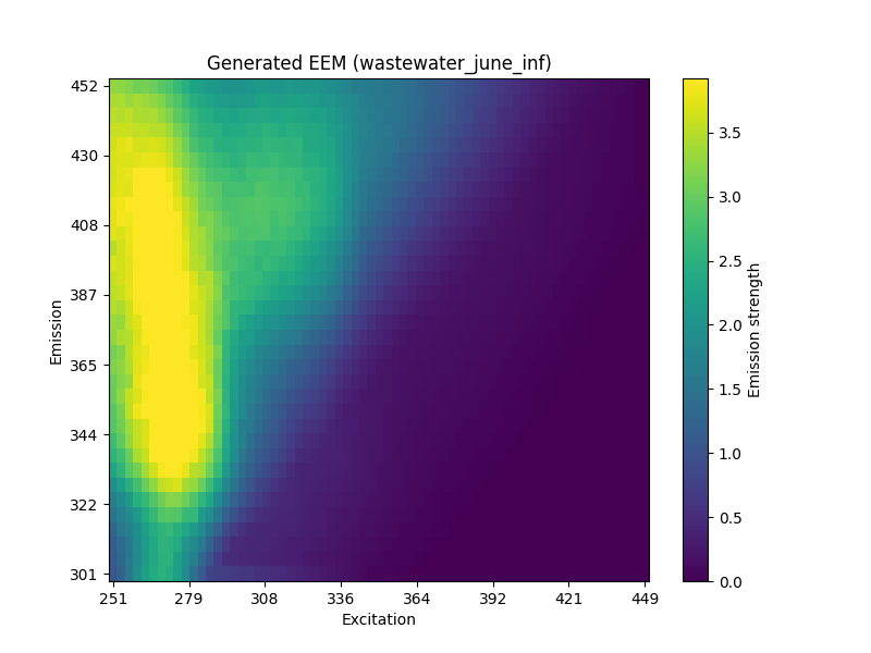
The generator is not evaluated with a single quantitative score in this report, but the qualitative outputs are useful for interpreting how changes in concentrations might shift fluorescence patterns. This makes the model a promising tool for hypothesis generation even before formal evaluation metrics are added.
Generative modeling is included because it addresses a different question than prediction. Instead of asking what metadata can be inferred from an EEM, it asks what EEM would be expected for a given metadata profile. This inversion of the prediction task can be useful for simulation studies or for understanding the sensitivity of the fluorescence surface to specific pollutants.
Because the generator is trained on the same reduced set of samples as the predictive models, its outputs should be interpreted within the same scope. It is best viewed as a proof of concept that links metadata to plausible EEM structure, rather than as a final model for scientific inference.
A useful next step for generative modeling would be to define clear evaluation metrics, such as reconstruction error on a held out set or similarity of generated spectra to measured spectra in key wavelength regions. Adding such metrics would help move the model from exploratory to quantitative assessment.
Another direction would be to use the generator to simulate new sample conditions, such as intermediate concentration levels that are not present in the training data. This could help visualize how the fluorescence surface changes smoothly with concentration and could guide future experimental design.
6 Limitations and Assumptions
Some source categories, especially within natural water subsets, have small sample counts. This reduces statistical power and can inflate variance in cross validation and permutation testing. The non-significant natural Kung versus natural Del result is consistent with this limitation.
The preprocessing step fills scatter bands and missing grid points. While necessary for uniform modeling, interpolation can smooth local peaks and may reduce sensitivity to subtle spectral features. This is mitigated by focusing on global structure in PCA and by comparing raw versus preprocessed heatmaps.
Principal component analysis is a linear reduction and may not capture all non-linear relationships present in raw EEM grids. The success of the MLP suggests that non-linear structure remains in the reduced space, but some information is still inevitably lost.
The reported results are tied to the specific preprocessing and model choices used in this project. Alternative preprocessing strategies, such as different interpolation schemes or wavelength ranges, could change the downstream modeling outcomes. This highlights the importance of documenting each step clearly.
The models also assume that the metadata labels are accurate and consistent. Any errors in the metadata would directly affect both training and evaluation, which is a general limitation in supervised learning pipelines.
7 Possible Future Development
As mentioned in Section 5, a variational autoencoder was used for the generative modelling but it could also be used to replace PCA and be trained jointly with prediction, potentially yielding a reduced representation more aligned with the regression and classification objectives. This would incorporate everything together in one incredibly versatile model.
The source paper uses parallel factor analysis models to remove background fluorescence and isolate micropollutant signals. Integrating a similar pre step could improve interpretability and enhance sensitivity to subtle spiking effects, especially at low concentrations.
The conditional EEM generator can be strengthened with improved architectures, regularization, and evaluation criteria. For example, comparing generated EEMs to held out real spectra, or conditioning on additional metadata, could make the model a useful tool for simulation studies or sensitivity analysis.
Future work could also include uncertainty estimation for concentration predictions, which would help quantify confidence in model outputs and make the results more actionable for experimental design.
Another future direction is to test whether adding raw wavelength regions or alternative features improves model performance. This could include combining PCA features with summary statistics from the original EEMs, which might capture additional information not preserved in the linear reduction.
8 Conclusion
This project demonstrates that fluorescence EEM data contain usable predictive information about micropollutant spiking and sample origin. A careful preprocessing pipeline and PCA preserve the dominant structure in the data, and visual inspection confirms that spiking gradients align with systematic trajectories in principal component space. Permutation tests show that differences between sources are statistically significant in most comparisons, reinforcing the validity of the reduced features.
In predictive modeling, the multitask MLP achieves excellent regression performance and strong classification accuracy, while random forests provide robust, high accuracy classification at the cost of weaker regression. The models are therefore complementary. The MLP is better suited to quantitative spiking estimates, and the random forest is attractive for source classification when interpretability and robustness are priorities.
Finally, the generative model offers a constructive view of how metadata and source labels map back to fluorescence patterns, extending the analysis beyond discriminative prediction. Together, these results suggest that EEM based modeling can provide practical, low cost insights into micropollutant behavior and water source differences, consistent with the findings and motivations of the original study.
9 References
- (1) Paradina-Fernandez, L.; Wunsch, U.; Bro, R.; Murphy, K. Direct measurement of organic micropollutants in water and wastewater using fluorescence spectroscopy. ACS EST Water 2023, 3, 3905–3915. https://doi.org/10.1021/acsestwater.3c00323.
- (2) McKinney, W. Data structures for statistical computing in Python. In Proceedings of the 9th Python in Science Conference; 2010; pp 56–61.
- (3) Harris, C. R., Millman, K. J., van der Walt, S. J., et al. Array programming with NumPy. Nature 2020, 585, 357–362.
- (4) Virtanen, P., Gommers, R., Oliphant, T. E., et al. SciPy 1.0: fundamental algorithms for scientific computing in Python. Nat. Methods 2020, 17, 261–272.
- (5) Hunter, J. D. Matplotlib: a 2D graphics environment. Comput. Sci. Eng. 2007, 9, 90–95.
- (6) Plotly Technologies Inc. Plotly Graphing Libraries. https://plotly.com/graphing-libraries/ (accessed 2026-01-24).
- (7) Paszke, A., Gross, S., Massa, F., et al. PyTorch: an imperative style, high-performance deep learning library. In Advances in Neural Information Processing Systems 32; 2019; pp 8024–8035.
- (8) Pedregosa, F., Varoquaux, G., Gramfort, A., et al. Scikit-learn: machine learning in Python. J. Mach. Learn. Res. 2011, 12, 2825–2830.
Download and Run the Code
You can clone the repository or download it as a zip file, then run the pipeline script to rebuild the processed data, figures, and model results.
Zip download: https://github.com/meli-mckeown/MultivariateDataAnalysis/archive/refs/heads/main.zip
Clone and run:
git clone git@github.com:meli-mckeown/MultivariateDataAnalysis.git
cd MultivariateDataAnalysis
bash everything.sh
Python packages that may be required:
python3 -m pip install torch matplotlib plotly numpy pandas scikit-learn scipy richAdditional packages may be required depending on your environment and Python version.
Read everything.sh to see the individual steps and how to tweak
them for faster execution or to skip the full grid search.